Interpolation, approximation and differential equations solvers

Contents

Problem 1

1.1 Problem definition

1.2 Solution of the problem

1.2.1 Linear interpolation

1.2.2 Method of least squares interpolation

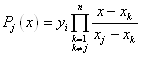
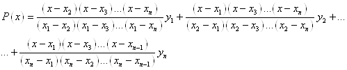
1.2.3 Lagrange interpolating polynomial

1.2.4 Cubic spline interpolation

1.3 Results and discussion

1.3.1 Lagrange polynomial

Problem 2

2.1 Problem definition

2.2 Problem solution

2.2.1 Rectangular method

2.2.2 Trapezoidal rule

2.2.3 Simpson's rule

2.2.4 Gauss-Legendre method and Gauss-Chebyshev method

Problem 3

3.1 Problem definition

3.2 Problem solution

Problem 4

4.1 Problem definition

4.2 Problem solution

References

Problem 1   1.1 Problem definition

For the following data set, please discuss the possibility of obtaining a reasonable interpolated value at , , and  via at least 4 different interpolation formulas you are have learned in this semester.

  1.2 Solution of the problem

Interpolation is a method of constructing new data points within the range of a discrete set of known data points.

In engineering and science one often has a number of data points, as obtained by sampling or experimentation, and tries to construct a function which closely fits those data points. This is called curve fitting or regression analysis. Interpolation is a specific case of curve fitting, in which the function must go exactly through the data points.

First we have to plot data points, such plot provides better picture for analysis than data arrays

Following four interpolation methods will be discussed in order to solve the problem:

·  Linear interpolation

·  Method of least squares interpolation

·  Lagrange interpolating polynomial

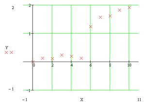
Fig 1. Initial data points

·  Cubic spline interpolation

  1.2.1 Linear interpolation

One of the simplest methods is linear interpolation (sometimes known as lerp). Generally, linear interpolation tales two data points, say  and , and the interpolant is given by:

 at the point

Linear interpolation is quick and easy, but it is not very precise/ Another disadvantage is that the interpolant is not differentiable at the point .

1.2.2 Method of least squares interpolation

The method of least squares is an alternative to interpolation for fitting a function to a set of points. Unlike interpolation, it does not require the fitted function to intersect each point. The method of least squares is probably best known for its use in statistical regression, but it is used in many contexts unrelated to statistics.

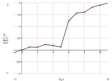
Fig 2. Plot of the data with linear interpolation superimposed

Generally, if we have  data points, there is exactly one polynomial of degree at most  going through all the data points. The interpolation error is proportional to the distance between the data points to the power n. Furthermore, the interpolant is a polynomial and thus infinitely differentiable. So, we see that polynomial interpolation solves all the problems of linear interpolation.

However, polynomial interpolation also has some disadvantages. Calculating the interpolating polynomial is computationaly expensive compared to linear interpolation. Furthermore, polynomial interpolation may not be so exact after all, especially at the end points. These disadvantages can be avoided by using spline interpolation.

Example of construction of polynomial by least square method

Data is given by the table:

Polynomial is given by the model:

In order to find the optimal parameters  the following substitution is being executed:

, , …,

Then:

The error function:

It is necessary to find parameters , which provide minimums to function :

It should be noted that the matrix  must be nonsingular matrix.

For the given data points matrix  become singular, and it makes impossible to construct polynomial with  order, where  - number of data points, so we will use  polynomial

Fig 3. Plot of the data with polynomial interpolation superimposed

Because the polynomial is forced to intercept every point, it weaves up and down.

  1.2.3 Lagrange interpolating polynomial

The Lagrange interpolating polynomial is the polynomial  of degree  that passes through the  points , , …,  and is given by:

,

Where

Written explicitly

When constructing interpolating polynomials, there is a tradeoff between having a better fit and having a smooth well-behaved fitting function. The more data points that are used in the interpolation, the higher the degree of the resulting polynomial, and therefore the greater oscillation it will exhibit between the data points. Therefore, a high-degree interpolation may be a poor predictor of the function between points, although the accuracy at the data points will be "perfect."

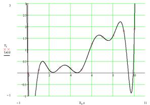
Fig 4. Plot of the data with Lagrange interpolating polynomial interpolation superimposed

One can see, that Lagrange polynomial has a lot of oscillations due to the high order if polynomial.